I teach the undergraduate solid state physics course, where we just switched to a shiny new book "Oxford Solid State Basics" by Steve Simon.

Steve's story of condensed matter physics starts with the heat capacity of solid materials. It's a great way to dive into how quantum mechanics combines with lucky guesses to improve our understanding of what is happening. It is also what we do in our course.

A great source of experimental data showing the problem is Einstein's original work, and Steve's book reproduces the plot from Einstein. (See also the English translation) Unfortunately that plot belongs to the current publisher of Annalen der Physik and cannot be republished under a free license. So in order to provide this data in the lecture notes and to make it available to whoever wants, I decided to take the original data Einstein has and repeat the exercise. Because we are living in an enlightened age, I also wanted to see if the more advanced Debye model would be any better for Einstein's data.

Here's the source table from Einstein's work. (By the way, find a typo ;)

einstein's original data

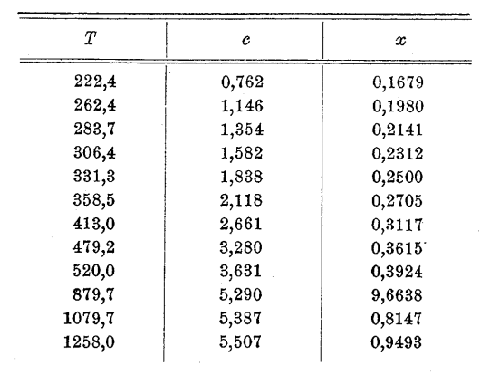
Let's analyse it!

# Once again the basic imports that we'll need later

from matplotlib import pyplot
import numpy as np
from scipy.optimize import curve_fit
from scipy.integrate import quad

pyplot.rcParams['figure.figsize'] = (10, 7)
pyplot.rcParams['font.size'] = 20

To get the data from the drawing I decided to use the Tesseract OCR library:

data = !tesseract einstein_data.png stdout -l eng

Unfortunately, with all the simplicity of use, Tesseract makes a handful of mistakes which we have to correct manually.

data = np.array([float(i.replace(',', '.').replace('s', '5')) for i in data if i.strip()])
T, c = data[:12], data[12:24]

c[7] = 3.28
c[-2] = 5.387
c[4] = 1.838
T[-3] = 879.7
T[2] = 283.7
T[-1] = 1258

print(list(T), list(c))

[222.4, 262.4, 283.7, 306.4, 331.3, 358.5, 413.0, 479.2, 520.0, 879.7, 1079.7, 1258.0] [0.762, 1.146, 1.354, 1.582, 1.838, 2.118, 2.661, 3.28, 3.631, 5.29, 5.387, 5.507]

Deviation from the Dulong–Petit law¶

The simplest theory of heat capacity of solids is the Dulong–Petit law saying that each atom has 6 degrees of freedom (3x kinetic and 3x potential), and therefore heat capacity per atom is $C = 6 \times 1/2 = 3$ (in units of Boltzmann constant). Afterwards experiments observed that at low temperatures the Dulong–Petit law breaks down and heat capacity drops.

Einstein was measuring heat capacities in gram-calories; we start by translating it into natural units and plotting the original data.

Just like Einstein in his time we see something very different from a temperature-independent heat capacity.

c *= 3 / 5.96

def plot_data():
    pyplot.scatter(T, c)
    pyplot.xlim(xmin=0)
    pyplot.ylim(0, 3)
    pyplot.xlabel('$T [K]$')
    pyplot.ylabel('$C/k_B$')

plot_data()

Einstein solid (fitting the data)¶

Einstein (Steve explains that Einstein was a pretty smart guy in his book) came up with an idea to model each atom as a quantum harmonic oscillator (Einstein solid), which explained the heat capacity reduction using the quantum mechanics (which didn't exist yet).

Einstein's model predicted the following law: $$ C_V = 3 (T_E/T)^2 \frac{e^{T_E/T}}{(e^{T_E/T} - 1)^2}, $$ with the temperature scale $T_E = \hbar \omega/k_B$ a model parameter.

Having the data and the model, we just perform the fit and get the temperature scale of the einstein solid as a result.

def c_einstein(T, T_E):
    x = T_E / T
    return 3 * x**2 * np.exp(x) / (np.exp(x) - 1)**2

fit = curve_fit(c_einstein, T, c, 1000)
T_E = fit[0][0]
delta_T_E = np.sqrt(fit[1][0, 0])
print(f"T_E = {T_E:.5} ± {delta_T_E:.3} K")

plot_data()
temps = np.linspace(10, T[-1], 100)
pyplot.plot(temps, c_einstein(temps, T_E));

T_E = 1295.8 ± 14.7 K

Curiously, Einstein's original curve looks visibly different.

Einstein's figure

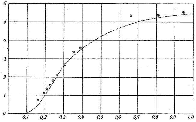
The resolution to the mystery is rather simple: Einstein didn't make an actual fit, he just matched a single point!

Quoting from his work:

For T = 331.3 we have c = 1.838; according to the theory described, from this it follows that A = 11.0μ.

And indeed, it's easy to find the very point Einstein used to perform the "fit", and where the curve intersects with the data. Those were simple times :)

Debye model¶

Einstein's model was still not good enough and Debye improved it by considering heat capacity of sound waves with a linear dispersion.

As one last fun exercise we will check if the more advanced Debye model explains the data better.

The Debye heat capacity is

$$ C_V = 9 (T/T_D)^3 \int_0^{T_D/T} \frac{x^4 e^x}{(e^x - 1)^2}dx $$

def integrand(y):
    return y**4 * np.exp(y) / (np.exp(y) - 1)**2

@np.vectorize
def c_debye(T, T_D):
    x = T / T_D
    return 9 * x**3 * quad(integrand, 0, 1/x)[0]

fit = curve_fit(c_debye, T, c, 1000)
T_D = fit[0][0]
delta_T_D = np.sqrt(fit[1][0, 0])
print(f"T_D = {T_D:.5} ± {delta_T_D:.3} K")

plot_data()
pyplot.plot(temps, c_einstein(temps, T_E), label='Einstein')
pyplot.plot(temps, c_debye(temps, T_D), label='Debye')
pyplot.legend();

T_D = 1788.7 ± 27.6 K

So with the data Einstein used one couldn't really tell the difference.

Summary¶

We took a table from Einstein's paper, processed it, plotted, and improved on Einstein's work by making an actual least squares fit. Next I will include this in my course notes and also discuss how one publishes course notes altogether.